What Is It?
Weibull analysis is a time-to-failure method used to describe how a population of non-repairable items survives over time. Its shape parameter can represent decreasing, roughly constant, or increasing failure hazard, while its scale parameter sets a characteristic time. Fitted to failure and properly recorded still-operating equipment, it can estimate survival probabilities and support maintenance planning. It does not identify the exact failure time of an individual asset, and the model is only useful when its assumptions fit the failure mechanism and data.
Why Does It Matter for Cities?
Cities and utilities depend on fleets of pumps, electrical equipment, luminaires, controls, and building systems. A time-to-failure model can help teams compare maintenance intervals, prepare spares, or prioritize inspection when asset histories are available. The value is a better-informed plan—not a promise that a particular pump or controller will fail on a predicted date.
Where Is It Used?
- Estimating failure probability for water pumps, motors, valves, and other utility assets
- Planning inspection or preventive-replacement intervals for distribution equipment
- Reviewing streetlighting, HVAC, and traffic-control component life histories
- Estimating whether a series, redundant, or k-out-of-n configuration meets a defined mission-time reliability target
- Supporting maintenance workload and spare-parts forecasts from a documented asset population
Evidence note
The guide explains how Weibull analysis can support asset-reliability planning, but the reviewed SCD sources do not document a named municipal deployment of this method. The examples elsewhere on this page are potential applications, not evidence that a city uses Weibull analysis.
Illustrative scenario
How Might It Be Applied?
Illustrative only: suppose a non-repairable component population is modeled with β = 2 and η = 10 operating-years. At five years, estimated survival is about 77.9% and cumulative failure probability is about 22.1%. The instantaneous hazard is 0.10 per year at that age. For a unit that has already survived five years, the modeled probability of failure during the following year is about 10.4%. These are population-model outputs, not a forecast for a named asset or evidence from a city deployment.
How Does It Work?
- 01Define the item, failure mode, time origin, exposure unit, and event that counts as failure; use operating hours or cycles when calendar age is not the relevant exposure.
- 02Assemble each unit's time to failure or last known operating time, including right-censored units that had not failed when observation ended. Record repairs, removals, environment, and operating conditions.
- 03Fit shape (β) and scale (η), commonly by maximum likelihood for censored data, then examine probability plots, confidence bounds, residual patterns, and alternative lifetime models.
- 04Calculate survival, cumulative failure probability, hazard, and conditional risk over the actual planning interval. Translate population-level estimates into a maintenance decision only after considering costs, service consequences, and uncertainty.
What Information Does It Need?
Benefits
- Flexible shape can represent decreasing, constant, or increasing population hazard
- Survival methods can use both observed failures and appropriately censored observations
- Results can be carried into time-dependent series and redundancy calculations
- Probability estimates can help make maintenance and inventory decisions explicit
Limitations and Risks
- A Weibull fit is not proof that Weibull is the right lifetime model; multiple distributions may fit sparse data similarly.
- Failure mechanisms, asset cohorts, exposure, repairs, and reporting practices may differ; pooling them can produce misleading parameters.
- Standard series, parallel, and k-out-of-n formulas assume suitable component independence and a correctly defined system success condition.
- Common-cause failures, dependent loads, switching faults, dormant standby failures, and repair can invalidate simple block calculations.
- Reliability is probability of surviving a stated mission interval; availability also depends on repair and restoration time.
Weibull fundamentals: survival, failure, density, and hazard
For the two-parameter Weibull model, t is a nonnegative exposure time, β > 0 is shape, and η > 0 is scale (characteristic life). At t = η, the model has accumulated 1 − e⁻¹, or about 63.2%, probability of failure. The model assumes a zero location threshold; a shifted three-parameter form is a different, more demanding model and should not be adopted just to improve fit.
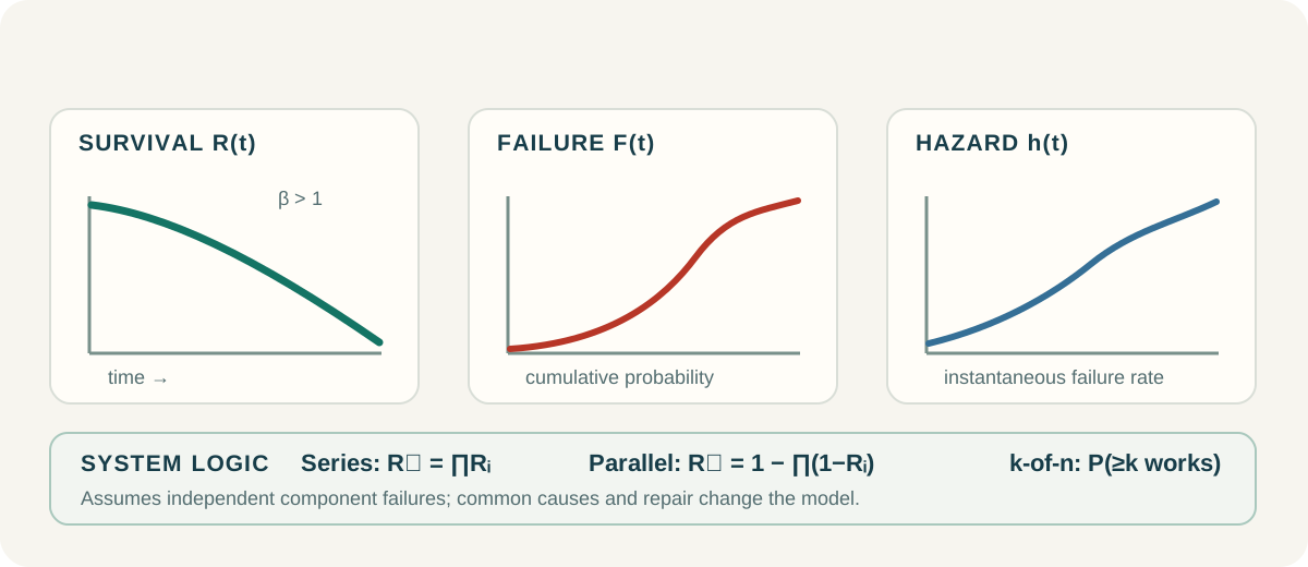
The shape parameter describes how the population's instantaneous hazard changes with age. β < 1 gives a decreasing hazard, sometimes called an infant-mortality pattern; β = 1 gives constant hazard and the exponential distribution; β > 1 gives increasing hazard, often consistent with wear-out. These patterns describe fitted populations and do not by themselves explain a physical cause.
Survival / reliability: R(t) = exp[−(t / η)^β]
Cumulative failure probability: F(t) = 1 − R(t)
Probability density: f(t) = (β / η)(t / η)^(β−1) exp[−(t / η)^β]
Time-dependent hazard: h(t) = f(t) / R(t) = (β / η)(t / η)^(β−1)
Mean time to first failure: E[T] = η Γ(1 + 1 / β)
Estimating parameters from failures and censored equipment
A failure observation contributes its failure time; a right-censored observation contributes the fact that the item survived at least to its last observation time. For independent, non-informative right censoring, the two-parameter likelihood combines the density for each observed failure with the survival probability for each censored unit. Maximum likelihood estimation can fit β and η without pretending censored units failed at the date monitoring stopped.
For observation i, let tᵢ be its recorded failure or censoring exposure, and let δᵢ equal 1 for a failure and 0 for right censoring. Parameter uncertainty matters: report confidence intervals or bounds for β, η, and decision-relevant probabilities, using a suitable likelihood method or resampling approach. A point estimate alone can disguise weak evidence.
Before fitting, define the cohort and failure mode, verify timestamps and exposure units, and distinguish failures from planned removals or repairs. Check whether censoring is plausibly independent of failure risk. Truncation, interval-censored inspections, competing failure modes, changing maintenance, and mixed asset populations need methods that represent those conditions rather than being silently treated as simple right censoring.
Right-censored likelihood: L(β, η) = ∏ᵢ [f(tᵢ)]^δᵢ [R(tᵢ)]^(1−δᵢ)
Estimate (β, η) by maximizing L, or equivalently the log-likelihood; then assess fit and uncertainty.
- Use probability plots and diagnostic checks; a straight-looking Weibull plot is evidence to assess, not proof of model adequacy.
- Compare plausible alternatives such as exponential or lognormal models when data and failure physics warrant it.
- Validate predictions against a later period or held-out cohort when sample size permits; do not reuse the fitting sample as the only validation.
From a fitted curve to a planning interval
R(t) answers: what fraction of a comparable population is expected to survive to exposure t? F(t) is the complementary probability of a first failure by t. The density describes how probability is distributed over time; it is not itself a probability of failure at one exact instant. The hazard is an instantaneous conditional rate among units that have survived to t, with units inverse to the time unit.
For an asset already operating at age t, the probability of failure during the next Δ exposure units, conditional on survival to t, is not F(Δ). It is one minus the ratio of survival at t + Δ to survival at t. That distinction is important for age-based maintenance decisions.
An illustrative risk-threshold calculation can solve F(t) = q for t = η[−ln(1 − q)]^(1/β). With β = 2, η = 10 years, and a chosen 10% cumulative first-failure threshold, the model reaches that threshold at about 3.25 exposure-years. This is only a mathematical illustration: an acceptable risk threshold and replacement policy must come from engineering requirements, consequences, costs, and applicable standards—not from the Weibull curve alone.
Conditional interval risk: P(t < T ≤ t + Δ | T > t) = 1 − R(t + Δ) / R(t)
For β = 2, η = 10 years, and t = 5 years: R(5) = e^(−0.25) ≈ 0.779; F(5) ≈ 0.221
At t = 5: h(5) = 0.10 per year; one-year conditional risk = 1 − e^(−(0.6²−0.5²)) ≈ 0.104
System reliability: series, active parallel, mixed, and k-out-of-n
A reliability block diagram represents which component successes are required for the system to perform its defined function over a mission interval. The following formulas use each component's reliability Rᵢ(t) at the same interval and assume independent component survival unless stated otherwise. If component reliability is Weibull, substitute its Rᵢ(t) into the system formula; a resulting system distribution is not always itself Weibull.
Series: all n components must work → Rₛ(t) = ∏ᵢ Rᵢ(t)
Active parallel: at least one of n independent components must work → Rₚ(t) = 1 − ∏ᵢ[1 − Rᵢ(t)]
Mixed example: A in series with (B || C) → Rsys = R_A × [1 − (1 − R_B)(1 − R_C)]
Identical independent k-out-of-n: Rₖ/ₙ(t) = Σⱼ₌ₖⁿ C(n,j) R(t)^j [1 − R(t)]^(n−j)
- Series worked example: two independent components, each R = 0.98 over the mission, give Rₛ = 0.98² = 0.9604 (96.04%). A system fails when either required component fails.
- Active parallel worked example: two independent components, each R = 0.90, give Rₚ = 1 − 0.10² = 0.99 (99%). This assumes both are operating and either alone can carry the required load.
- Mixed worked example: A has R = 0.98 and either B or C (each 0.90) can provide the second block, so Rsys = 0.98 × [1 − 0.1²] = 0.9702 (97.02%).
- Two-out-of-three example: with three identical independent components each R = 0.90, the system succeeds if two or three work: C(3,2)(0.9²)(0.1) + C(3,3)(0.9³) = 0.972 (97.2%).
Practical limits, city applications, and maintenance decisions
Independence is often the fragile assumption. Components may share flood exposure, heat, power, software, maintenance crews, suppliers, communications, or environmental stress. A common-cause event can defeat redundant equipment at once; multiplying independent reliabilities would overstate protection. Standby redundancy also needs a separate model for dormant failures, proof-test coverage, switching demand and success, and the time to detect and transfer load. A standby unit is not equivalent to an active parallel unit.
Weibull lifetime models normally describe first failure of a non-repairable item or a defined first-failure population. After repair, the asset may be renewed, minimally repaired, or changed; repeated-event data then require a repairable-system or recurrent-event model. Reliability measures survival through a stated interval without failure. Availability measures the fraction of time service is operational and therefore depends on repair, restoration, logistics, and downtime as well as failure behavior.
In city operations, candidate assets include water pumps and valves, electrical transformers and switchgear, streetlighting drivers or luminaires, traffic-signal controllers, and HVAC motors or fans. Each use needs a carefully defined unit and failure mode: a lamp failure is not the same event as a corridor losing required lighting, and a component reliability estimate is not automatically a service-level reliability estimate.
For preventive maintenance, teams can compare modeled interval risk with inspection, replacement, labor, outage, and consequence costs, then evaluate sensitivity to parameter bounds. For spare parts, a fleet-level survival model can help estimate how many similar units may require service during supplier lead time. For reliability improvement, stratify by failure mode and exposure, test whether a design or maintenance change shifts the observed distribution, and monitor the result. All worked numbers on this page are illustrative calculations, not findings from actual city deployments or recommendations for a particular asset.
The linked Technology and Company Atlas entries describe relevant infrastructure and equipment contexts; they are not evidence that a named supplier or city uses Weibull analysis. No individual city project is connected here because the current SCD evidence does not document a named urban deployment of this specific method.
- Do not infer a precise failure date for an individual item from a population curve.
- Do not replace equipment solely because a Weibull β is above one; inspect the failure mechanism, uncertainty, and consequences.
- Do not interpret a low failure count as proof of high reliability when observation time, censoring, or sample size is limited.
- Keep observed deployment evidence, fitted statistical estimates, and hypothetical calculations clearly separate.
Explore Further
- Building management systems →
Explore building equipment and maintenance context.
- Smart City Atlas & Map →
Browse city profiles; current published evidence does not document a named city deployment of Weibull analysis.
Frequently Asked Questions
Does Weibull analysis predict the exact date a pump or controller will fail?
No. It estimates population survival and conditional probabilities. An individual asset's condition, use, and unobserved factors can differ.
Can still-operating equipment be used in the estimate?
Yes. Proper right-censored survival times contribute information that each item survived at least to its last observation. They should not be recorded as failures on that date.
Does β > 1 prove wear-out is the physical cause?
No. It indicates an increasing fitted population hazard under the model. Physical inspection and failure-mode evidence are needed to identify cause.
Does adding a parallel pump always make a system more reliable?
Only under a suitable architecture and assumptions. Capacity, independent failure, common causes, controls, switching, and maintenance all affect whether redundancy works.
Is reliability the same as availability?
No. Reliability is survival without failure over a stated interval. Availability also accounts for restoration and repair time.
Sources & References
- 01NIST/SEMATECH e-Handbook of Statistical Methods — Weibull Distribution and Reliability Formulas ↗
- 02NIST/SEMATECH e-Handbook — Estimating Life Distribution Parameters from Censored Data ↗
- 03NIST/SEMATECH e-Handbook — Weibull Maximum Likelihood Estimation Example ↗
- 04NIST/SEMATECH e-Handbook — Series Reliability Model ↗
- 05NIST/SEMATECH e-Handbook — Parallel or Redundant Reliability Model ↗
- 06NIST/SEMATECH e-Handbook — R-out-of-N Reliability Model ↗
- 07NIST/SEMATECH e-Handbook — Complex Reliability Systems ↗
- 08NIST/SEMATECH e-Handbook — Reliability or Survival Function ↗
Related Atlas links show documented topic or research connections. A cross-link alone does not establish that a named city or company deployed this specific method; deployment evidence and status are described in the project notes above.
Back to AI & Analytics Atlas →